

CSS cubic-bezier() Math: Control Points, Inversion, and Newton's Method
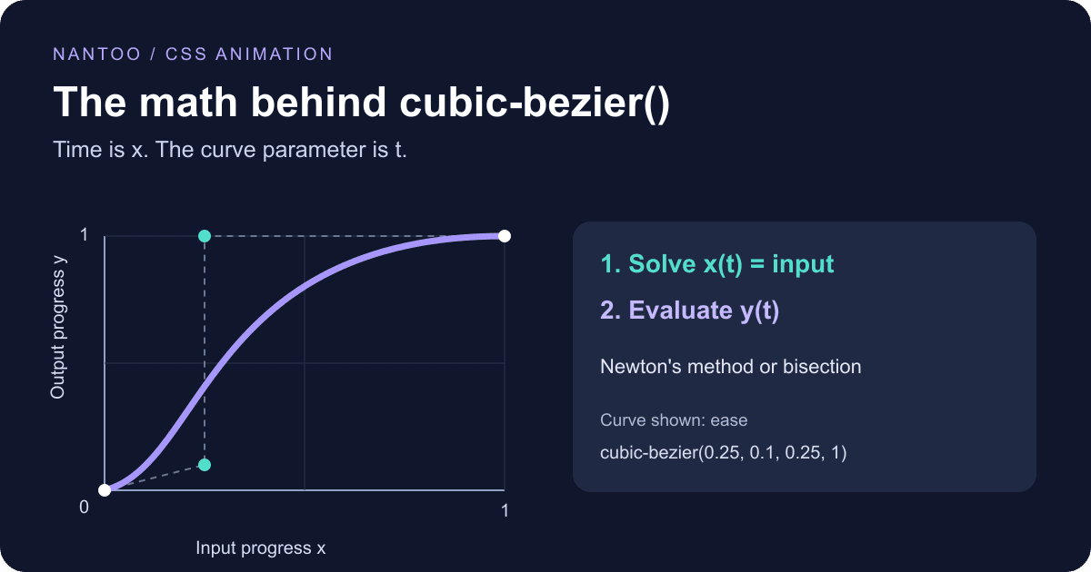
You have chosen cubic-bezier(0.25, 0.1, 0.25, 1.0) for a CSS transition. What do those four numbers actually control? Unlike an SVG path, which uses a Bézier curve to describe a shape, CSS uses the curve to map input progress to output progress. The endpoints stay at (0,0) and (1,1), and the two x control coordinates must lie between 0 and 1. This article explains the mathematics behind that restriction and the inverse problem solved by Newton–Raphson iteration or bisection. CSS Easing Functions defines the required output, without prescribing a particular numerical solver inside a browser.
Japanese original published: 2026-05-01
A Bézier curve as an easing function
An SVG path describes a shape in a plane. A CSS easing curve instead relates two quantities:
- x: input progress, typically normalized elapsed time from 0 at the start to 1 at the end.
- y: output progress used to interpolate the animated property between its start and end values.
The fixed endpoints are P₀=(0,0) and P₃=(1,1). The arguments to cubic-bezier(x1, y1, x2, y2) specify P₁=(x₁,y₁) and P₂=(x₂,y₂). Together, they define the one-dimensional mapping y=f(x).
The published CSS Easing Functions Level 2 Working Draft covers cubic Bézier easing in §2.3. The numerical discussion here concerns x ∈ [0,1]. CSS also defines output outside that interval by extending the curve using endpoint-side control points. The curve parameter t is not elapsed time; it is an intermediate value used to evaluate the curve.
The cubic equation and the Bernstein basis
Four control points define a cubic Bézier curve. For a parameter t between 0 and 1, its point B(t) is:
B(t) = (1-t)³ P₀ + 3(1-t)² t P₁ + 3(1-t) t² P₂ + t³ P₃The four weights are the cubic Bernstein basis polynomials. Their properties follow from the binomial expansion:
- Nonnegativity: Bᵢ,ₙ(t) ≥ 0 on [0,1].
- Partition of unity: the weights sum to 1.
- Symmetry: Bᵢ,ₙ(t)=Bₙ₋ᵢ,ₙ(1−t).
Nonnegative weights that sum to 1 make B(t) a convex combination of all four control points. The curve stays inside their convex hull, including the fixed endpoints. It need not stay between P₁ and P₂ alone. Since all four x coordinates lie in [0,1] for a valid CSS curve, x(t) stays within that interval too.
Why the x control coordinates must stay in [0,1]
With the endpoints fixed, the x coordinate simplifies to:
x(t) = 3(1-t)² t · x₁ + 3(1-t) t² · x₂ + t³To use the curve as a mapping from x to y, its x coordinate must not turn back on itself. Otherwise a single input could correspond to several curve parameters. Differentiating gives:
x'(t) = 3[(1-t)² x₁ + 2(1-t)t(x₂-x₁) + t²(1-x₂)]The restrictions x₁,x₂ ∈ [0,1] guarantee a nonnegative derivative. They do not require x₁ ≤ x₂. Here is a derivation: at a fixed t, x'(t)/3 is affine in the two control coordinates, so its value on their unit square is a convex combination of the values at the four corners:
(x₁, x₂) = (0, 0): x'(t)/3 = t²
(x₁, x₂) = (0, 1): x'(t)/3 = 2t(1-t)
(x₁, x₂) = (1, 0): x'(t)/3 = (1-2t)²
(x₁, x₂) = (1, 1): x'(t)/3 = (1-t)²
All four expressions are nonnegative. Also, x(t) is a nonconstant polynomial, so its derivative cannot vanish throughout a nonzero interval. Thus x(t) is strictly increasing, although its derivative can be zero at an individual point. For x₁=1 and x₂=0, that happens at t=0.5. The inverse is still unique.
The y control coordinates have no corresponding [0,1] restriction in CSS. For example, cubic-bezier(0.68, -0.55, 0.27, 1.55) can move below 0 and above 1, producing an undershoot and an overshoot.
The inverse problem: finding t from time
A browser needs output progress y for the current input progress x. But the parametric equation gives t → (x,y), not y directly from x. Substituting elapsed progress for t generally gives the wrong result.
- Solve x(t)=x for the curve parameter t.
- Evaluate y(t) at that parameter.
The first step is a cubic root-finding problem. An analytic solution is possible, but an implementation can instead choose an iterative method based on accuracy, cost, and behavior near difficult control points. The CSS specification does not require a particular root-finding algorithm.
Newton–Raphson iteration and bisection
Newton's method solves x(t)−x_target=0 by repeatedly applying:
t_next = t - (x(t) - x_target) / x'(t)A small derivative can send the next estimate outside [0,1]. A zero derivative can occur inside the interval as well as at an endpoint: x₁=1, x₂=0, t=0.5 is one example. A guarded solver checks the residual, derivative, proposed step, and iteration limit, and can fall back to bisection when Newton's method is unsafe.
Bisection halves the candidate parameter interval at each step. It often takes more iterations, but uses monotonicity to keep the root bracketed. NanToo's cubic-bezier editor uses 40 bisection steps for interior preview inputs and returns the endpoints directly for input progress 0 or 1. In exact real arithmetic the remaining interval has width 2⁻⁴⁰. That is not a guarantee of the same accuracy in y after floating-point rounding.
The editor's limits are separate from CSS syntax. It bounds x₁/x₂ to 0–1 and y₁/y₂ to −1–2, then rounds control coordinates to two decimal places. It also clamps input progress to 0–1. It is therefore a bounded preview tool, not a general evaluator for CSS extrapolation outside that interval.
Standard CSS easing keywords
The four ease keywords correspond to cubic Bézier curves. The separate linear keyword is an identity easing function; the final row shows a curve with the same y=x output.
Scroll horizontally if the table does not fit.
| Keyword | Control coordinates (x₁,y₁,x₂,y₂) | Behavior |
|---|---|---|
ease | (0.25, 0.1, 0.25, 1.0) | Slow start, faster middle, slow finish |
ease-in | (0.42, 0, 1.0, 1.0) | Starts slowly and accelerates |
ease-out | (0, 0, 0.58, 1.0) | Starts quickly and slows down |
ease-in-out | (0.42, 0, 0.58, 1.0) | Symmetric slow start and finish |
linear | (0, 0, 1.0, 1.0) | Equivalent constant-rate output |
The initial value of transition-timing-function is ease. For the diagonal curve in the linear row, x(t)=y(t), but neither coordinate generally equals t. Also distinguish the keyword linear from the linear() function, which interpolates between multiple points.
One cubic curve cannot express an arbitrary sequence of bounces: y'(t) is quadratic, so there can be at most two interior turning points. Depending on the motion you need, alternatives include a piecewise-linear approximation using linear(), multiple keyframes, or a custom JavaScript calculation.
Bézier curves in font outlines
The same family of curves also describes letter shapes, rather than timing.
Scroll horizontally if the table does not fit.
| Outline format | Curve degree | Points per segment | Origin |
|---|---|---|---|
| TrueType (Apple/Microsoft, 1991) | Quadratic | 3: start, control, end | Apple |
| OpenType CFF / Type 1 outlines | Cubic | 4: start, two controls, end | Adobe |
TrueType outlines use quadratic curves; CFF and Type 1 outlines use cubic curves. OpenType supports both quadratic and cubic outline representations. The approximation and subdivision algorithms inside a rasterizer can vary by implementation.
Horner evaluation versus de Casteljau interpolation
There are two useful ways to evaluate the curve at a known t. First, expand a coordinate into a polynomial and use Horner's method. For the fixed CSS x endpoints, this JavaScript computes x(t):
const a = 3 * x1 - 3 * x2 + 1;
const b = -6 * x1 + 3 * x2;
const c = 3 * x1;
const x = ((a * t + b) * t + c) * t;
After precomputing a, b, and c, one coordinate evaluation uses three multiplications and two additions. That count excludes coefficient setup and any iterations used to invert x(t).
Second, de Casteljau's algorithm repeatedly interpolates between adjacent points. Here lerp(A,B,t) means (1−t)A+tB, applied to each coordinate:
Q0 = lerp(P0, P1, t)
Q1 = lerp(P1, P2, t)
Q2 = lerp(P2, P3, t)
R0 = lerp(Q0, Q1, t)
R1 = lerp(Q1, Q2, t)
B  = lerp(R0, R1, t)
A cubic curve requires six interpolations, not necessarily six multiplications. For example, the scalar expression (1-t)*a+t*b uses two multiplications and one addition even if 1−t is already available. Horner evaluation is compact; actual speed also depends on the implementation and environment. De Casteljau interpolation is well suited to stable evaluation through convex combinations on [0,1], but neither method eliminates floating-point error.
Key points
- CSS uses a Bézier curve to map input progress to output progress.
- The endpoints are fixed; the four arguments specify the two interior control points.
- x₁,x₂ ∈ [0,1] guarantee a unique inverse, even when x₁ is greater than x₂.
- CSS permits y control coordinates outside [0,1], allowing overshoot.
- Finding t from x is a separate step from evaluating the curve at t.
- Newton's method needs guards; bisection uses the monotonic x coordinate to retain a bracket.
- The Bernstein basis keeps the curve in the convex hull of all control points, including the endpoints.
- The four ease keywords are cubic Bézier aliases; linear is a separate keyword with identity output.
- TrueType and CFF outlines illustrate quadratic and cubic Bézier curves in another setting.
References and sources
- W3C CSS Easing Functions Level 2 Working Draft — Cubic Bézier easing functions ↗
- W3C CSS Easing Functions Level 1 ↗
- W3C CSS Transitions Level 1 — transition-timing-function ↗
- Michigan Technological University — De Casteljau's Algorithm ↗
- Apple TrueType Reference Manual — Digitizing Letterform Designs ↗
- Adobe Type 1 Font Format — Charstrings ↗
Editorial note
This article was prepared with AI assistance and reviewed by an editor before publication. It may still contain factual errors, interpretation mistakes, or outdated information. Check the cited primary sources or official documentation before making an important decision.