

Image dithering explained: Bayer matrices, Floyd–Steinberg, GIF and ASCII art
When only a few colors are available, a gradient can turn into visible bands. Dithering changes the arrangement of dots to suggest intermediate brightness or color. It does not increase the number of stored colors: it trades spatial texture for the appearance of smoother tones.
GIF images do not necessarily use dithering, and ASCII art does not necessarily use error diffusion. This article compares Bayer ordered dithering with Floyd–Steinberg error diffusion, while separating palette selection, GIF compression and character mapping.
Japanese original published: 2026-04-26
Quantization and dithering do different jobs
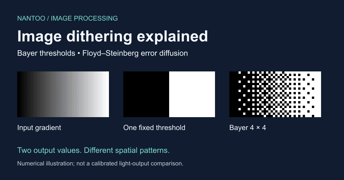
Quantization maps an input to a limited set of output values. In a black-and-white image, for example, each output pixel is either black or white. Applying one fixed threshold can turn a gradual gradient into large separate black and white areas.
Dithering varies the threshold by position or passes quantization error to unprocessed pixels, using dot density to suggest intermediate tones. At a viewing distance where fine patterns blend visually, the result can look smoother. Up close, grain or a regular pattern may be visible. Text and fine details can be easier to read without dithering; it is not an automatic quality improvement.
Applications include bilevel printing, palette images and conversion to lower bit depths. Saving with lossless compression, such as PNG compression, does not make a preceding color-reduction step lossless relative to the original. Dithering is not a reversible encoding of the original pixel values either.
Ordered dithering with a Bayer matrix
B. E. Bayer’s 1973 publication concerns rendering continuous-tone pictures with two output levels. Here we use a teaching model that repeats a 4×4 threshold matrix across a black-and-white image. Input values range from 0 to 255; white is 255 and black is 0. The following is explanatory pseudocode, not JavaScript that can be run as written. Coordinates start at zero: x increases to the right and y downward; % denotes the remainder.
D4 = [[0, 8, 2, 10],
      [12, 4, 14, 6],
      [3, 11, 1, 9],
      [15, 7, 13, 5]]
threshold = (D4[y % 4][x % 4] + 0.5) / 16
output = (input / 255 > threshold) ? 255 : 0
The thresholds lie at the centers of 16 intervals; this is not simply an endpoint-to-endpoint mapping of 0–15 onto 0–255. Input 0 makes every pixel black, input 255 makes every pixel white, and input 127.5 makes eight of the 16 pixels white. For a uniform input, the tile can contain 0–16 white pixels: 17 coverage levels. Each pixel still has only two possible values. This model describes numerical proportions; a 50% encoded RGB value does not necessarily represent 50% of the physical light output.
D1 = [[0]]
D(2n) = [[4*Dn,       4*Dn + 2*Un],
         [4*Dn+3*Un, 4*Dn +   Un]]
Un = an n × n matrix whose entries are all 1
Each term in the recurrence is an n×n matrix; the brackets describe a block matrix formed by placing those matrices side by side and above one another. This recurrence generates 2×2, 4×4 and 8×8 matrices. Each pixel depends only on its coordinates and input, making the calculation suitable for parallel execution on a GPU. A matrix fixed in screen coordinates does not guarantee flicker-free video: moving images and changing colors can still cross thresholds and change the visible pattern.
Floyd–Steinberg: error weights and image boundaries
Floyd and Steinberg’s 1976 paper is an original source for spatial error diffusion. In a left-to-right, top-to-bottom scan, quantize the current value v, including error already received, to obtain q. Then pass e = v − q to the following unprocessed pixels:
(x+1, y)   += e * 7/16
(x-1, y+1) += e * 3/16
(x,   y+1) += e * 5/16
(x+1, y+1) += e * 1/16
The weights add up to one, but they do not distribute the error equally. All of that error is passed on mathematically only when every destination exists and intermediate values are not rounded or clipped. An implementation that discards contributions outside the image loses error at its edges. The average of a finite output image need not exactly match the input average.
For example, take a 2×1 input [100, 100], white output for values greater than 127.5 and black output otherwise and a rule that discards error outside the image. The first pixel becomes black, 0, leaving error 100. Its right-hand neighbor becomes 100 + 100×7/16 = 143.75, so it is quantized to white, 255. The output is [0, 255], whose sum differs from the input sum of 200. A weight sum of one does not guarantee exact preservation of the entire image’s average.
Use floating-point values or another suitable representation to retain accumulated error. Storing each intermediate result in an 8-bit array, or clipping it to 0–255, can change the output. Scan order, boundary handling and rounding are part of the algorithm’s operating conditions.
Variants: where the error goes and how much is passed on
Jarvis–Judice–Ninke, Stucki, Burkes, Sierra and Atkinson use different error destinations or weights. Compare actual kernels and output instead of ranking methods by name or publication year. The table below checks three kernels in gif.js’s GIFEncoder.js. The sums assume that all destinations are inside the image.
Scroll horizontally if the table does not fit.
| Method | Destinations | Weight sum | What the kernel tells us |
|---|---|---|---|
| Floyd–Steinberg | 4 pixels, current and next row | 16/16 = 1 | Distributes error over a relatively small neighborhood |
| Stucki | 12 pixels, current and next two rows | 42/42 = 1 | Distributes error over a wider neighborhood |
| Atkinson | 6 pixels, current and next two rows | 6/8 = 3/4 | Passes 1/8 to each destination; does not pass on the remaining 1/4 |
Table source: GitHub: gif.js/src/GIFEncoder.js at master · jnordberg/gif.js. This checks implementation weights; it does not establish the invention date of each method.
A larger neighborhood means more pixel accesses and updates, but not necessarily a better-looking result. Partial diffusion, as in Atkinson, can lose subtle tonal distinctions. Compare photographs, edges and any intended retro appearance in the actual output.
Color quantization and GIF: choose a palette, then assign colors
With an arbitrary color palette, color reduction first selects the available colors and then assigns pixels to palette entries. Rounding RGB channels independently can produce combinations that are not in the palette. That is different from selecting an output color from the palette and diffusing the input-minus-output difference as a color vector.
Results depend on the color-distance metric and on whether errors are calculated in linear light or encoded RGB. Naming CIEDE2000 or OKLab does not guarantee a better result: the required color-space conversions and evaluation for the intended purpose still matter. See the article on CSS color-mix() and OKLCH for more on color spaces.
pngquant combines palette generation with adaptive dithering. A simple four-step description of RGB nearest-neighbor mapping plus standard Floyd–Steinberg is not a complete description of that implementation.
A GIF color table has at most 256 entries. Images with local color tables can have their own palettes, so an entire animation need not use one common set of 256 colors. Dithering is not required by the GIF specification, and it is separate from LZW compression. The article on GIF and LZW patents explains that distinction further.
NanToo’s GIF maker uses gif.js, but its current invocation does not specify dithering and the default is false. A library supporting Floyd–Steinberg and other methods is different from a tool enabling those features.
ASCII art: character mapping is not error diffusion
A character set ordered from visually dense to sparse can map brightness to character selection. However, perceived density depends on the font, spacing, foreground and background. N characters do not guarantee N perceptually equal tone steps. An image looking recognizable through character density is not evidence that it uses Floyd–Steinberg.
NanToo’s ASCII art converter composites transparent pixels onto white and rounds each resulting channel before applying the following weights and index mapping. This is also pseudocode. N is the number of entries in a character set, at least two; idx is a zero-based index, and floor rounds down. R, G and B are the composited values on a 0–255 scale.
L = 0.299*R + 0.587*G + 0.114*B
mapped = invert ? 255-L : L
idx = min(N-1, max(0, floor(mapped/255 * (N-1))))
This is a brightness approximation using BT.601 luma coefficients. Applying those coefficients to Canvas RGB values does not implement the whole BT.601 signal-processing system, nor does it measure physical luminance in linear light.
Black maps to the first character and white to the last; the invert option reverses the brightness mapping. The current conversion does not use error diffusion. Several character sets are available, so it would be inaccurate to claim that it always reproduces 256 tones faithfully using 70 characters. Evaluate the character sequence together with its actual font rendering.
Patterns, scan direction and compression trade-offs
Error diffusion can still produce regular textures or streaks. Serpentine scanning reverses direction on alternate rows; a right-to-left row also requires the kernel’s horizontal offsets to be mirrored. This can reduce directional bias, but it does not guarantee the removal of visible patterns.
Ordered dithering reuses the threshold at each coordinate, but its repeated tile can become visible. Blue-noise threshold arrangements and curve-following error diffusion such as Riemersma provide other options. ImageMagick offers Riemersma and Floyd–Steinberg error diffusion as well as ordered dithering. A product name alone does not establish that every mode uses the same kernel or scan order.
Adding fine variations to a flat area can increase the compressed file size. Dithering balances apparent tone, edge clarity, grain, processing time and storage size; it does not create additional information for free.
Lower bit depths and GPU execution
When a high-precision image is quantized to a lower bit depth, dithering is one option for making banding less conspicuous. HDR-to-SDR tone mapping changes the brightness range, however, and is not synonymous with changing numerical precision from 16 to 8 bits. Design tone mapping, gamut conversion, quantization and dithering as distinct steps.
The Bayer formula depends on a pixel’s coordinates and input, so it can run in parallel on a GPU. Ordinary error diffusion makes later pixels depend on earlier results. This distinction affects the implementation strategy.
Spatial image dithering, temporal sampling and INT8 quantization of machine-learning models all involve finite representations, but they are not the same algorithm. That shared theme does not establish that Floyd–Steinberg or Bayer dithering is generally used in AI inference, or that either is close to an information-theoretic optimum.
Summary: change the arrangement, not the number of colors
- Quantization limits output values; dithering changes patterns to alter the appearance of intermediate tones.
- Bayer uses coordinate-dependent thresholds. Floyd–Steinberg quantizes a value that includes accumulated error, then distributes the new error with unequal weights.
- A weight sum of one does not guarantee exact preservation of the average when boundaries, rounding or clipping intervene.
- GIF palette limits, dithering during color reduction and LZW compression are separate mechanisms.
- ASCII character mapping and error diffusion are also distinct. Check the implementation, settings and font.
- Compare grain, edges, processing speed and file size on images representative of the intended use.
References and sources
- JST J-GLOBAL: An adaptive algorithm for spatial greyscale. ↗(Floyd and Steinberg, 1976, Proc. SID 17(2):75–77. Bibliographic information, not access to the full paper.)
- Wikipedia: Ordered dithering - Wikipedia ↗
- Computer Graphics and Image Processing: A survey of techniques for the display of continuous tone pictures on bilevel displays ↗
- Wikipedia: Error diffusion ↗
- mitpress.mit.edu: Digital Halftoning ↗
- ACM Transactions on Graphics: Digital halftones by dot diffusion ↗
- ITU: BT.601 : Studio encoding parameters of digital television for standard 4:3 and wide screen 16:9 aspect ratios ↗
- Network: Computation in Neural Systems: Kohonen neural networks for optimal colour quantization ↗
- NDL Search: An Optimum Method for Two-Level Rendition of Continuous-Tone Pictures ↗(Bayer, 1973. Bibliographic information, not the full paper.)
- CompuServe: Graphics Interchange Format, Version 89a ↗
- GitHub: gif.js/src/GIFEncoder.js at master · jnordberg/gif.js ↗
- pngquant: pngquant ↗
- ImageMagick: Command-line Options ↗
- Joel Yliluoma: Joel Yliluoma's arbitrary-palette positional dithering algorithm ↗
Editorial note
This article was prepared with AI assistance and reviewed by an editor before publication. It may still contain factual errors, interpretation mistakes, or outdated information. Check the cited primary sources or official documentation before making an important decision.